Diffusion Models
What is diffusion?
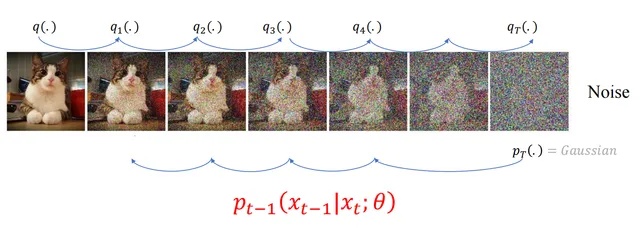
Inspired by physical diffusion, DDPM uses a fixed forward process that gradually adds Gaussian noise while attenuating the original signal. This transforms a complex data distribution into a distribution close to the standard Gaussian N ( 0 , I ) \mathcal{N}(0,I) N ( 0 , I )
A neural network learns to reverse this process step by step, allowing us to generate new data samples starting from Gaussian noise.
Diffusion models share a similar high-level idea with VAEs: both generate data from a simple latent distribution.
This leads to three challenges:
How do we define and simulate the forward diffusion process?
How do we model the reverse denoising process?
How do we train the model?
Forward process
The forward process adds Gaussian noise while attenuating the original signal, finally transforming the complex data distribution into a distribution close to the standard Gaussian N ( 0 , I ) \mathcal{N}(0,I) N ( 0 , I )
Starting from x 0 ∼ q 0 x_0\sim q_0 x 0 ∼ q 0 x t ∼ q t x_t\sim q_t x t ∼ q t q t q_t q t t t t
At each step:
q ( x t ∣ x t − 1 ) = N ( x t ; 1 − β t x t − 1 , β t I ) , x t = 1 − β t x t − 1 + β t ϵ t , ϵ t ∼ N ( 0 , I ) . \begin{aligned}
q(x_t\mid x_{t-1})
&=\mathcal N\!\left(x_t;\sqrt{1-\beta_t}\,x_{t-1},\beta_t I\right),\\
x_t
&=\sqrt{1-\beta_t}\,x_{t-1}+\sqrt{\beta_t}\,\epsilon_t,
\qquad \epsilon_t\sim\mathcal N(0,I).
\end{aligned} q ( x t ∣ x t − 1 ) x t = N ( x t ; 1 − β t x t − 1 , β t I ) , = 1 − β t x t − 1 + β t ϵ t , ϵ t ∼ N ( 0 , I ) .
Here, β t ∈ ( 0 , 1 ) \beta_t\in(0,1) β t ∈ ( 0 , 1 ) ϵ t \epsilon_t ϵ t
Direct sampling from x 0 x_0 x 0
q ( x t ∣ x 0 ) = N ( x t ; α t x 0 , ( 1 − α t ) I ) , x t = α t x 0 + 1 − α t ϵ , ϵ ∼ N ( 0 , I ) . \begin{aligned}
q(x_t\mid x_0)
&=\mathcal N\!\left(x_t;\sqrt{\alpha_t}\,x_0,(1-\alpha_t)I\right),\\
x_t
&=\sqrt{\alpha_t}\,x_0+\sqrt{1-\alpha_t}\,\epsilon,
\qquad \epsilon\sim\mathcal N(0,I).
\end{aligned} q ( x t ∣ x 0 ) x t = N ( x t ; α t x 0 , ( 1 − α t ) I ) , = α t x 0 + 1 − α t ϵ , ϵ ∼ N ( 0 , I ) .
Here, α t = ∏ s = 1 t ( 1 − β s ) \alpha_t=\prod_{s=1}^{t}(1-\beta_s) α t = ∏ s = 1 t ( 1 − β s ) α T ≈ 0 \alpha_T\approx0 α T ≈ 0 q T ≈ N ( 0 , I ) q_T\approx\mathcal N(0,I) q T ≈ N ( 0 , I )
Backward process
Starting from Gaussian noise,
x T ∼ p T , p T = N ( 0 , I ) , q T ≈ p T . x_T\sim p_T,\qquad p_T=\mathcal N(0,I),\qquad q_T\approx p_T. x T ∼ p T , p T = N ( 0 , I ) , q T ≈ p T . the reverse process generates data through successive denoising steps:
p θ ( x t − 1 ∣ x t ) = N ( x t − 1 ; μ θ ( x t , t ) , σ t 2 I ) , x t − 1 = μ θ ( x t , t ) + σ t z t , z t ∼ N ( 0 , I ) . \begin{aligned}
p_\theta(x_{t-1}\mid x_t)
&=\mathcal N\!\left(x_{t-1};\mu_\theta(x_t,t),\sigma_t^2I\right),\\
x_{t-1}
&=\mu_\theta(x_t,t)+\sigma_t z_t,
\qquad z_t\sim\mathcal N(0,I).
\end{aligned} p θ ( x t − 1 ∣ x t ) x t − 1 = N ( x t − 1 ; μ θ ( x t , t ) , σ t 2 I ) , = μ θ ( x t , t ) + σ t z t , z t ∼ N ( 0 , I ) . Here, x t ∼ p t x_t\sim p_t x t ∼ p t p θ ( x 0 ) p_\theta(x_0) p θ ( x 0 ) p 0 ( x 0 ) p_0(x_0) p 0 ( x 0 )
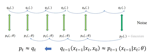
A shared network predicts μ θ ( x t , t ) \mu_\theta(x_t,t) μ θ ( x t , t ) σ t 2 \sigma_t^2 σ t 2 p t ≈ q t p_t\approx q_t p t ≈ q t p 0 ≈ q 0 p_0\approx q_0 p 0 ≈ q 0
The marginals q t q_t q t p t p_t p t
DDPM training
Diffusion ELBO
Maximize the expected log-likelihood:
max θ E q 0 ( x 0 ) [ log p θ ( x 0 ) ] ⟺ min θ E q 0 ( x 0 ) [ − log p θ ( x 0 ) ] . \max_\theta\;
\mathbb E_{q_0(x_0)}[\log p_\theta(x_0)]
\quad\Longleftrightarrow\quad
\min_\theta\;
\mathbb E_{q_0(x_0)}[-\log p_\theta(x_0)]. θ max E q 0 ( x 0 ) [ log p θ ( x 0 )] ⟺ θ min E q 0 ( x 0 ) [ − log p θ ( x 0 )] . Let z = ( x 1 , … , x T ) z=(x_1,\ldots,x_T) z = ( x 1 , … , x T )
p θ ( x 0 ) = ∫ p θ ( x 0 , z ) d z . p_\theta(x_0)=\int p_\theta(x_0,z)\,dz. p θ ( x 0 ) = ∫ p θ ( x 0 , z ) d z . Use the fixed forward distribution:
q ( z ∣ x 0 ) = ∏ t = 1 T q ( x t ∣ x t − 1 ) , q ( x 0 , z ) = q 0 ( x 0 ) q ( z ∣ x 0 ) . q(z\mid x_0)=\prod_{t=1}^{T}q(x_t\mid x_{t-1}),
\qquad
q(x_0,z)=q_0(x_0)q(z\mid x_0). q ( z ∣ x 0 ) = t = 1 ∏ T q ( x t ∣ x t − 1 ) , q ( x 0 , z ) = q 0 ( x 0 ) q ( z ∣ x 0 ) . Write E q \mathbb E_q E q q ( x 0 , z ) q(x_0,z) q ( x 0 , z ) z z z
E q 0 ( x 0 ) [ − log p θ ( x 0 ) ] = E q [ − log p θ ( x 0 ) ] . \mathbb E_{q_0(x_0)}[-\log p_\theta(x_0)]
=
\mathbb E_q[-\log p_\theta(x_0)]. E q 0 ( x 0 ) [ − log p θ ( x 0 )] = E q [ − log p θ ( x 0 )] . Insert q ( z ∣ x 0 ) / q ( z ∣ x 0 ) q(z\mid x_0)/q(z\mid x_0) q ( z ∣ x 0 ) / q ( z ∣ x 0 )
p θ ( x 0 ) = p θ ( x 0 , z ) p θ ( z ∣ x 0 ) . p_\theta(x_0)
=
\frac{p_\theta(x_0,z)}{p_\theta(z\mid x_0)}. p θ ( x 0 ) = p θ ( z ∣ x 0 ) p θ ( x 0 , z ) . Then
E q 0 [ − log p θ ( x 0 ) ] = E q [ − log ( q ( z ∣ x 0 ) q ( z ∣ x 0 ) p θ ( x 0 ) ) ] = E q [ − log ( q ( z ∣ x 0 ) q ( z ∣ x 0 ) p θ ( x 0 , z ) p θ ( z ∣ x 0 ) ) ] = E q [ − log q ( z ∣ x 0 ) p θ ( z ∣ x 0 ) ] + E q [ − log p θ ( x 0 , z ) q ( z ∣ x 0 ) ] . \begin{aligned}
\mathbb E_{q_0}[-\log p_\theta(x_0)]
&=
\mathbb E_q\left[
-\log\left(
\frac{q(z\mid x_0)}{q(z\mid x_0)}
p_\theta(x_0)
\right)
\right]\\[4pt]
&=
\mathbb E_q\left[
-\log\left(
\frac{q(z\mid x_0)}{q(z\mid x_0)}
\frac{p_\theta(x_0,z)}{p_\theta(z\mid x_0)}
\right)
\right]\\[4pt]
&=
\mathbb E_q\left[
-\log\frac{q(z\mid x_0)}{p_\theta(z\mid x_0)}
\right]
+
\mathbb E_q\left[
-\log\frac{p_\theta(x_0,z)}{q(z\mid x_0)}
\right].
\end{aligned} E q 0 [ − log p θ ( x 0 )] = E q [ − log ( q ( z ∣ x 0 ) q ( z ∣ x 0 ) p θ ( x 0 ) ) ] = E q [ − log ( q ( z ∣ x 0 ) q ( z ∣ x 0 ) p θ ( z ∣ x 0 ) p θ ( x 0 , z ) ) ] = E q [ − log p θ ( z ∣ x 0 ) q ( z ∣ x 0 ) ] + E q [ − log q ( z ∣ x 0 ) p θ ( x 0 , z ) ] . By KL nonnegativity:
E q [ − log q ( z ∣ x 0 ) p θ ( z ∣ x 0 ) ] = − E q 0 [ D K L ( q ( z ∣ x 0 ) ∥ p θ ( z ∣ x 0 ) ) ] ≤ 0. \mathbb E_q\left[
-\log\frac{q(z\mid x_0)}{p_\theta(z\mid x_0)}
\right]
=
-\mathbb E_{q_0}\left[
D_{\mathrm{KL}}\!\left(
q(z\mid x_0)\,\|\,p_\theta(z\mid x_0)
\right)
\right]
\le0. E q [ − log p θ ( z ∣ x 0 ) q ( z ∣ x 0 ) ] = − E q 0 [ D KL ( q ( z ∣ x 0 ) ∥ p θ ( z ∣ x 0 ) ) ] ≤ 0. Thus,
E q 0 [ − log p θ ( x 0 ) ] ≤ E q [ − log p θ ( x 0 , z ) q ( z ∣ x 0 ) ] , E q 0 [ log p θ ( x 0 ) ] ≥ E q [ log p θ ( x 0 , z ) q ( z ∣ x 0 ) ] . \begin{aligned}
\mathbb E_{q_0}[-\log p_\theta(x_0)]
&\le
\mathbb E_q\left[
-\log\frac{p_\theta(x_0,z)}{q(z\mid x_0)}
\right],\\[4pt]
\mathbb E_{q_0}[\log p_\theta(x_0)]
&\ge
\mathbb E_q\left[
\log\frac{p_\theta(x_0,z)}{q(z\mid x_0)}
\right].
\end{aligned} E q 0 [ − log p θ ( x 0 )] E q 0 [ log p θ ( x 0 )] ≤ E q [ − log q ( z ∣ x 0 ) p θ ( x 0 , z ) ] , ≥ E q [ log q ( z ∣ x 0 ) p θ ( x 0 , z ) ] . This lower bound is the ELBO . We minimize its negative:
ELBO ( θ ) : = E q [ log p θ ( x 0 , z ) q ( z ∣ x 0 ) ] , L V L B ( θ ) : = − ELBO ( θ ) = E q [ − log p θ ( x 0 , z ) q ( z ∣ x 0 ) ] . \begin{aligned}
\operatorname{ELBO}(\theta)
&:=\mathbb E_q\left[
\log\frac{p_\theta(x_0,z)}{q(z\mid x_0)}
\right],\\[4pt]
\mathcal L_{\mathrm{VLB}}(\theta)
&:=-\operatorname{ELBO}(\theta)
=\mathbb E_q\left[
-\log\frac{p_\theta(x_0,z)}{q(z\mid x_0)}
\right].
\end{aligned} ELBO ( θ ) L VLB ( θ ) := E q [ log q ( z ∣ x 0 ) p θ ( x 0 , z ) ] , := − ELBO ( θ ) = E q [ − log q ( z ∣ x 0 ) p θ ( x 0 , z ) ] . Factorize the paths:
p θ ( x 0 , z ) = p T ( x T ) ∏ t = 1 T p θ ( x t − 1 ∣ x t ) , p_\theta(x_0,z)
=
p_T(x_T)\prod_{t=1}^{T}p_\theta(x_{t-1}\mid x_t), p θ ( x 0 , z ) = p T ( x T ) t = 1 ∏ T p θ ( x t − 1 ∣ x t ) , q ( z ∣ x 0 ) = q ( x T ∣ x 0 ) ∏ t = 2 T q ( x t − 1 ∣ x t , x 0 ) . q(z\mid x_0)
=
q(x_T\mid x_0)
\prod_{t=2}^{T}q(x_{t-1}\mid x_t,x_0). q ( z ∣ x 0 ) = q ( x T ∣ x 0 ) t = 2 ∏ T q ( x t − 1 ∣ x t , x 0 ) . Substitute:
L V L B = E q [ − log p θ ( x 0 ∣ x 1 ) + log q ( x T ∣ x 0 ) p T ( x T ) + ∑ t = 2 T log q ( x t − 1 ∣ x t , x 0 ) p θ ( x t − 1 ∣ x t ) ] . \begin{aligned}
\mathcal L_{\mathrm{VLB}}
=
\mathbb E_q\Bigg[
&-\log p_\theta(x_0\mid x_1)
+\log\frac{q(x_T\mid x_0)}{p_T(x_T)}\\
&+\sum_{t=2}^{T}
\log\frac{
q(x_{t-1}\mid x_t,x_0)
}{
p_\theta(x_{t-1}\mid x_t)
}
\Bigg].
\end{aligned} L VLB = E q [ − log p θ ( x 0 ∣ x 1 ) + log p T ( x T ) q ( x T ∣ x 0 ) + t = 2 ∑ T log p θ ( x t − 1 ∣ x t ) q ( x t − 1 ∣ x t , x 0 ) ] . Taking conditional expectations gives:
L V L B = E q [ − log p θ ( x 0 ∣ x 1 ) ] ⏟ reconstruction + ∑ t = 2 T E q [ D K L ( q ( x t − 1 ∣ x t , x 0 ) ∥ p θ ( x t − 1 ∣ x t ) ) ] ⏟ denoising + E q 0 [ D K L ( q ( x T ∣ x 0 ) ∥ p T ( x T ) ) ] ⏟ prior matching . \begin{aligned}
\mathcal L_{\mathrm{VLB}}
={}&
\underbrace{
\mathbb E_q[-\log p_\theta(x_0\mid x_1)]
}_{\text{reconstruction}}\\
&+
\underbrace{
\sum_{t=2}^{T}
\mathbb E_q\left[
D_{\mathrm{KL}}\!\left(
q(x_{t-1}\mid x_t,x_0)
\,\|\,
p_\theta(x_{t-1}\mid x_t)
\right)
\right]
}_{\text{denoising}}\\
&+
\underbrace{
\mathbb E_{q_0}\left[
D_{\mathrm{KL}}\!\left(
q(x_T\mid x_0)\,\|\,p_T(x_T)
\right)
\right]
}_{\text{prior matching}}.
\end{aligned} L VLB = reconstruction E q [ − log p θ ( x 0 ∣ x 1 )] + denoising t = 2 ∑ T E q [ D KL ( q ( x t − 1 ∣ x t , x 0 ) ∥ p θ ( x t − 1 ∣ x t ) ) ] + prior matching E q 0 [ D KL ( q ( x T ∣ x 0 ) ∥ p T ( x T ) ) ] . Drop the prior term, which is constant in θ \theta θ
min θ E q [ − log p θ ( x 0 ∣ x 1 ) + ∑ t = 2 T D K L ( q ( x t − 1 ∣ x t , x 0 ) ∥ p θ ( x t − 1 ∣ x t ) ) ] . \boxed{
\min_\theta\;
\mathbb E_q\left[
-\log p_\theta(x_0\mid x_1)
+
\sum_{t=2}^{T}
D_{\mathrm{KL}}\!\left(
q(x_{t-1}\mid x_t,x_0)
\,\|\,
p_\theta(x_{t-1}\mid x_t)
\right)
\right].
} θ min E q [ − log p θ ( x 0 ∣ x 1 ) + t = 2 ∑ T D KL ( q ( x t − 1 ∣ x t , x 0 ) ∥ p θ ( x t − 1 ∣ x t ) ) ] .
Intuition: By minimizing the expected KL divergence between q ( x t − 1 ∣ x t , x 0 ) q(x_{t-1}\mid x_t,x_0) q ( x t − 1 ∣ x t , x 0 ) p θ ( x t − 1 ∣ x t ) p_\theta(x_{t-1}\mid x_t) p θ ( x t − 1 ∣ x t ) p t ≈ q t p_t\approx q_t p t ≈ q t
Reparameterization
For t ≥ 2 t\ge2 t ≥ 2
q ( x t − 1 ∣ x t , x 0 ) = N ( x t − 1 ; μ ~ t ( x t , x 0 ) , β ~ t I ) , q(x_{t-1}\mid x_t,x_0)
=\mathcal N\!\left(x_{t-1};\tilde\mu_t(x_t,x_0),\tilde\beta_t I\right), q ( x t − 1 ∣ x t , x 0 ) = N ( x t − 1 ; μ ~ t ( x t , x 0 ) , β ~ t I ) , μ ~ t ( x t , x 0 ) = α t − 1 β t 1 − α t x 0 + 1 − β t ( 1 − α t − 1 ) 1 − α t x t , β ~ t = 1 − α t − 1 1 − α t β t . \tilde\mu_t(x_t,x_0)
=\frac{\sqrt{\alpha_{t-1}}\beta_t}{1-\alpha_t}x_0
+\frac{\sqrt{1-\beta_t}(1-\alpha_{t-1})}{1-\alpha_t}x_t,
\qquad
\tilde\beta_t=\frac{1-\alpha_{t-1}}{1-\alpha_t}\beta_t. μ ~ t ( x t , x 0 ) = 1 − α t α t − 1 β t x 0 + 1 − α t 1 − β t ( 1 − α t − 1 ) x t , β ~ t = 1 − α t 1 − α t − 1 β t . With fixed variances, the KL loss becomes a weighted mean error:
D K L ( q ( x t − 1 ∣ x t , x 0 ) ∥ p θ ( x t − 1 ∣ x t ) ) = 1 2 σ t 2 ∥ μ ~ t ( x t , x 0 ) − μ θ ( x t , t ) ∥ 2 2 + C t , D_{\mathrm{KL}}\!\left(
q(x_{t-1}\mid x_t,x_0)\,\|\,p_\theta(x_{t-1}\mid x_t)
\right)
=\frac{1}{2\sigma_t^2}
\left\|\tilde\mu_t(x_t,x_0)-\mu_\theta(x_t,t)\right\|_2^2+C_t, D KL ( q ( x t − 1 ∣ x t , x 0 ) ∥ p θ ( x t − 1 ∣ x t ) ) = 2 σ t 2 1 ∥ μ ~ t ( x t , x 0 ) − μ θ ( x t , t ) ∥ 2 2 + C t , where C t C_t C t θ \theta θ
Express x 0 x_0 x 0
x t = α t x 0 + 1 − α t ϵ , ϵ ∼ N ( 0 , I ) , x 0 = x t − 1 − α t ϵ α t . \begin{aligned}
x_t&=\sqrt{\alpha_t}\,x_0+\sqrt{1-\alpha_t}\,\epsilon,
\qquad \epsilon\sim\mathcal N(0,I),\\
x_0&=\frac{x_t-\sqrt{1-\alpha_t}\,\epsilon}{\sqrt{\alpha_t}}.
\end{aligned} x t x 0 = α t x 0 + 1 − α t ϵ , ϵ ∼ N ( 0 , I ) , = α t x t − 1 − α t ϵ . Substitute into the target mean, using α t = ( 1 − β t ) α t − 1 \alpha_t=(1-\beta_t)\alpha_{t-1} α t = ( 1 − β t ) α t − 1
μ ~ t ( x t , x 0 ) = α t − 1 β t 1 − α t x t − 1 − α t ϵ α t + 1 − β t ( 1 − α t − 1 ) 1 − α t x t = 1 1 − β t ( x t − β t 1 − α t ϵ ) . \begin{aligned}
\tilde\mu_t(x_t,x_0)
&=\frac{\sqrt{\alpha_{t-1}}\beta_t}{1-\alpha_t}
\frac{x_t-\sqrt{1-\alpha_t}\,\epsilon}{\sqrt{\alpha_t}}
+\frac{\sqrt{1-\beta_t}(1-\alpha_{t-1})}{1-\alpha_t}x_t\\[4pt]
&=\frac{1}{\sqrt{1-\beta_t}}
\left(x_t-\frac{\beta_t}{\sqrt{1-\alpha_t}}\epsilon\right).
\end{aligned} μ ~ t ( x t , x 0 ) = 1 − α t α t − 1 β t α t x t − 1 − α t ϵ + 1 − α t 1 − β t ( 1 − α t − 1 ) x t = 1 − β t 1 ( x t − 1 − α t β t ϵ ) . Let the network predict ϵ θ ( x t , t ) \epsilon_\theta(x_t,t) ϵ θ ( x t , t )
μ θ ( x t , t ) = 1 1 − β t ( x t − β t 1 − α t ϵ θ ( x t , t ) ) . \mu_\theta(x_t,t)
=\frac{1}{\sqrt{1-\beta_t}}
\left(x_t-\frac{\beta_t}{\sqrt{1-\alpha_t}}\epsilon_\theta(x_t,t)\right). μ θ ( x t , t ) = 1 − β t 1 ( x t − 1 − α t β t ϵ θ ( x t , t ) ) . The mean error becomes a noise prediction error:
1 2 σ t 2 ∥ μ ~ t ( x t , x 0 ) − μ θ ( x t , t ) ∥ 2 2 = β t 2 2 σ t 2 ( 1 − β t ) ( 1 − α t ) ∥ ϵ − ϵ θ ( x t , t ) ∥ 2 2 . \frac{1}{2\sigma_t^2}
\left\|\tilde\mu_t(x_t,x_0)-\mu_\theta(x_t,t)\right\|_2^2
=
\frac{\beta_t^2}{2\sigma_t^2(1-\beta_t)(1-\alpha_t)}
\left\|\epsilon-\epsilon_\theta(x_t,t)\right\|_2^2. 2 σ t 2 1 ∥ μ ~ t ( x t , x 0 ) − μ θ ( x t , t ) ∥ 2 2 = 2 σ t 2 ( 1 − β t ) ( 1 − α t ) β t 2 ∥ ϵ − ϵ θ ( x t , t ) ∥ 2 2 . Removing the time-dependent weights and applying noise prediction at all steps gives
L s i m p l e ( θ ) = E x 0 , t , ϵ [ ∥ ϵ − ϵ θ ( α t x 0 + 1 − α t ϵ , t ) ∥ 2 2 ] , \boxed{
\mathcal L_{\mathrm{simple}}(\theta)
=
\mathbb E_{x_0,t,\epsilon}\left[
\left\|
\epsilon-\epsilon_\theta\!\left(
\sqrt{\alpha_t}\,x_0+\sqrt{1-\alpha_t}\,\epsilon,t
\right)
\right\|_2^2
\right],
} L simple ( θ ) = E x 0 , t , ϵ [ ϵ − ϵ θ ( α t x 0 + 1 − α t ϵ , t ) 2 2 ] , where x 0 ∼ q 0 x_0\sim q_0 x 0 ∼ q 0 t ∼ U n i f o r m { 1 , … , T } t\sim\mathrm{Uniform}\{1,\ldots,T\} t ∼ Uniform { 1 , … , T } ϵ ∼ N ( 0 , I ) \epsilon\sim\mathcal N(0,I) ϵ ∼ N ( 0 , I )
Intuition: Predict the added noise, then use it to compute the denoising mean.