Autoregressive (AR) Models

An autoregressive (AR) model represents a joint distribution as a product of conditional distributions, predicting each element given the preceding elements:

$$p_\theta(x_1,\ldots,x_n) = \prod_{i=1}^{n} p_\theta(x_i\mid x_1,\ldots,x_{i-1}),$$

where the first factor is $p_\theta(x_1)$. It generates samples one element at a time.

Training objective: Minimize the average negative log-likelihood over the training data. For one sequence:

$$\mathcal{L}(\theta;x) = -\log p_\theta(x_1,\ldots,x_n) = -\sum_{i=1}^{n}\log p_\theta(x_i\mid x_{<i}),$$

where $x_{<i}=(x_1,\ldots,x_{i-1})$. During training, each prediction is conditioned on the observed prefix (teacher forcing).

Evaluation: Perplexity is the exponential of the average token-level negative log-likelihood on held-out data.

$$\operatorname{PPL}(x) = \exp\left(\frac{\mathcal{L}(\theta;x)}{n}\right).$$

Lower perplexity is better when evaluated on the same data with the same tokenization.

Generation: Sample one element at a time, conditioned on the previously generated elements:

$$\hat{x}_i\sim p_\theta(\,\cdot\mid \hat{x}_{<i}).$$

Start from an empty sequence or a given prompt, and append each sampled element. Stop when an end-of-sequence token is generated or the specified length is reached.

Alternatively, greedy decoding selects the most probable next token at each step:

$$\hat{x}_i = \arg\max_v p_\theta(v\mid\hat{x}_{<i}).$$

Autoregressive models can be implemented in various ways, including n-gram models and fixed-window models. Among these approaches, RNNs and Transformers are two effective and well-known choices.

RNN-Based Autoregressive Models

An RNN updates its hidden state using the previous state and the current token, then uses the updated state to predict the next token:

$$h_t = f_W(h_{t-1}, x_t)$$

Here, $h_t$ is used to predict $x_{t+1}$.

The architecture is as follows.

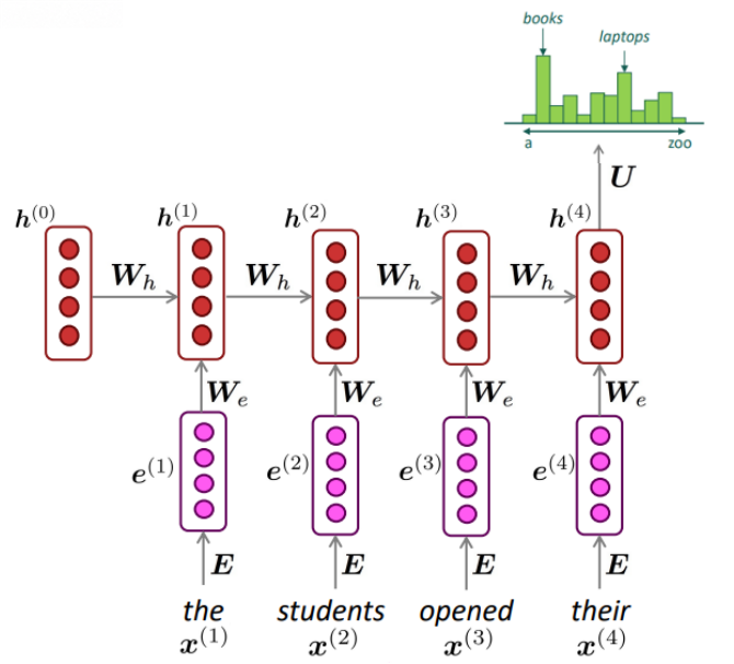
Unlike fixed-window models, RNNs can carry information beyond a fixed context window through their hidden states, although their ability to retain long-range information is limited.

Transformer-Based Autoregressive Models

A decoder-only Transformer combines causal self-attention, feed-forward layers, and positional information to model next-token distributions.

For input representations $X$, define $Q=XW_Q$, $K=XW_K$, and $V=XW_V$. Each attention head computes:

$$\operatorname{Attention}(Q,K,V) = \operatorname{softmax}\left( \frac{QK^\top}{\sqrt{d_k}}+M \right)V,$$

where $d_k$ is the key dimension.

To predict the next token $x_{i+1}$ using only $x_1,\ldots,x_i$, we add a causal mask to the attention scores before softmax. This blocks attention to future tokens and prevents information leakage during training.

$$M_{ij}= \begin{cases} 0, & j\le i,\\ -\infty, & j>i. \end{cases}$$

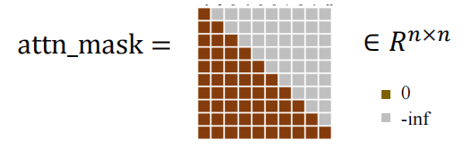
The final representation $h_t$ is used to predict $x_{t+1}$:

$$p_\theta(\,\cdot\mid x_{\le t}) = \operatorname{softmax}(W_o h_t+b_o).$$

Computational Complexity Comparison

Let $n$ be the sequence length. Assume fixed model size, full causal attention, and generation from an empty prefix.

Model	Training: total cost	Generation: cost at step $t$	Generation: total cost
RNN	$O(n)$	$O(1)$	$O(n)$
Transformer	$O(n^2)$	$O(t)$	$O(n^2)$

Generation reuses the RNN hidden state or a Transformer KV cache.

Training: RNNs process positions sequentially. Transformers can process positions in parallel during teacher-forced training, enabling efficient GPU computation despite their higher total operation count.

Generation: Both models generate tokens sequentially. Their total costs are:

$$T_{\mathrm{RNN}}=\sum_{t=1}^{n}O(1)=O(n), \qquad T_{\mathrm{Transformer}}=\sum_{t=1}^{n}O(t)=O(n^2).$$

Without KV caching, recomputing a full Transformer forward pass over every prefix instead costs $\sum_{t=1}^{n}O(t^2)=O(n^3)$.