Lecture 5: Image Stitching

1. Image Transformations

• Image warping changes the domain of images (pixel coordinates), while image filtering changes the range of images (pixel values).
• We use homogeneous coordinates to represent linear transformations and translations using matrix multiplication.

Affine Transformation: Linear Transformation plus Translation

We can use a matrix with 6 degrees of freedom to represent a linear transformation plus translation:

$$\begin{bmatrix}x'\\y'\\1\end{bmatrix} = \begin{bmatrix}a&b&t_x\\c&d&t_y\\0&0&1\end{bmatrix} \begin{bmatrix}x\\y\\1\end{bmatrix}, \qquad \mathbf{x}'=M\mathbf{x}+\mathbf{t}_0.$$

Here,

$$M=\begin{bmatrix}a&b\\c&d\end{bmatrix}, \qquad \mathbf{t}_0=\begin{bmatrix}t_x\\t_y\end{bmatrix}.$$

The fixed last row already removes the overall scale ambiguity.

In real applications, we can find many more point correspondences. We seek the optimal parameters by least squares:

$$E(\mathbf{t})=\|A\mathbf{t}-\mathbf{b}\|_2^2, \qquad \mathbf{t}^{*}=(A^TA)^{-1}A^T\mathbf{b}.$$

• t = (a, b, tₓ, c, d, tᵧ)ᵀ contains all six parameters.
• Stack the following two equations for each correspondence to build the 2n × 6 matrix A and the 2n-dimensional vector b:

$$\begin{bmatrix} x_i&y_i&1&0&0&0\\ 0&0&0&x_i&y_i&1 \end{bmatrix}\mathbf{t} =\begin{bmatrix}x_i'\\y_i'\end{bmatrix}.$$

• Condition: A must have full column rank for the inverse formula; at least 3 correspondences with non-collinear source points are required. An invertible affine transformation also requires det(M) ≠ 0.

Homography

A homography is more general than an affine transformation. We use a nonsingular 3 × 3 matrix H:

$$\tilde{\mathbf{x}}'\sim H\tilde{\mathbf{x}}, \qquad H=\begin{bmatrix} h_{11}&h_{12}&h_{13}\\ h_{21}&h_{22}&h_{23}\\ h_{31}&h_{32}&h_{33} \end{bmatrix}.$$

• Homogeneous coordinates use (x, y, 1)ᵀ; ∼ means equality up to nonzero scale. Divide the transformed coordinates by their third component, if nonzero, to obtain (x′, y′).
• 8 degrees of freedom: H and cH, for any c ≠ 0, represent the same transformation: 9 − 1 = 8.
• Stack two equations per correspondence to obtain A_H h = 0, where A_H is a 2n × 9 matrix and h contains the nine entries of H.
• Set ‖h‖₂ = 1 to fix the scale magnitude and exclude the trivial solution h = 0.

$$\min_{\|\mathbf{h}\|_2=1} E(\mathbf{h}), \qquad E(\mathbf{h})=\|A_H\mathbf{h}\|_2^2.$$

Using Lagrange multipliers gives

$$A_H^TA_H\mathbf{h}=\mu\mathbf{h}, \qquad E=\mu.$$

So h is a unit eigenvector of A_Hᵀ A_H with the smallest eigenvalue. This minimizes algebraic error.

• Minimum: 4 correspondences in general position (no three points collinear in either image).
• Applicability: a planar scene, or two camera views sharing the same optical center (pure rotation).

2. Feature Matching and RANSAC

We have a set of matches to build the panorama, where correct and wrong matches coexist. To reduce the influence of outliers, we use RANSAC (RANdom SAmple Consensus).

1. Randomly choose a minimal, non-degenerate subset of matches (4 for a homography).
2. Fit a model to the sampled matches.
3. Evaluate the model on all matches and find its inliers.
4. Repeat and choose the model with the largest set of inliers.
5. Refit the model using all selected inliers.

How to find inliers: use geometric error. For example, the forward reprojection error is

$$r_i=\|\mathbf{x}'_i-T_H(\mathbf{x}_i)\|_2, \qquad \text{inlier if }r_i\le\tau.$$

T_H includes homogeneous division. Choose τ according to localization noise and image scale; it is measured in pixels for pixel coordinates.

When to terminate: under the standard independent-sampling approximation,

$$P(\text{no all-inlier sample})=(1-G^P)^N, \qquad N_{\min}=\left\lceil\frac{\log\varepsilon}{\log(1-G^P)}\right\rceil.$$

• N: number of iterations; G: inlier ratio, 0 < G < 1; P: sample size; ε: allowed failure probability, 0 < ε < 1.
• Example: G = 0.5, P = 4, ε = 0.01 gives N_min = 72.
• This controls the probability of sampling an all-inlier subset, not a guarantee of a correct final model.

3. Image Blending

Image Blending with Laplacian Pyramid

Key idea: blend lower frequency bands over larger spatial ranges, and higher frequency bands over smaller spatial ranges.

Build Laplacian pyramids for both images and a Gaussian pyramid for the mask. Blend corresponding levels:

$$L_{\mathrm{out},k}=M_kL_{A,k}+(1-M_k)L_{B,k}.$$

Mₖ is the Gaussian mask at level k; multiplication is elementwise. Reconstruct from the blended coarsest base by repeatedly upsampling and adding the next finer blended detail level.

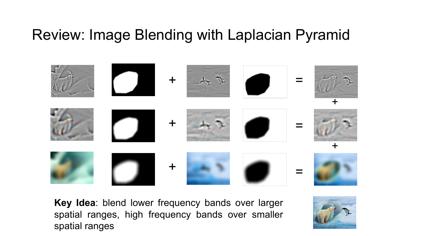
Source: Lecture 5, slide 29. From top to bottom, lower frequency bands use wider mask transitions.

Poisson Image Editing

We use Poisson image editing when the tones of the source image are not compatible with the target image.

Key idea: preserve source gradients as closely as possible while matching target pixel values on the region boundary.

$$\min_f\sum_{(i,j)\in\Omega} \|\nabla f(i,j)-\nabla g(i,j)\|_2^2, \qquad f|_{\partial\Omega}=f^*|_{\partial\Omega}.$$

• g: source image; f*: target image; f: output image; Ω: blending region.
• Gradients describe local changes such as edges and texture. Boundary pixel values, rather than gradients, are fixed; interior pixel values are solved for.

Matrix form (with pixel values flattened into vectors; solve each color channel separately):

$$\min_{\mathbf{f}}\|A\mathbf{f}-G\|_2^2 \quad\text{subject to}\quad B\mathbf{f}=F.$$

• A: neighboring-pixel difference matrix; G = Ag: source gradients.
• B: boundary selection matrix; F: target pixel values on the boundary.

The slide uses a penalty formulation:

$$\min_{\mathbf{f}}\|A\mathbf{f}-G\|_2^2 +\lambda\|B\mathbf{f}-F\|_2^2, \qquad \lambda>0.$$

Setting the derivative to zero gives the sparse linear system:

$$(A^TA+\lambda B^TB)\mathbf{f} =A^TG+\lambda B^TF.$$

• Finite λ encourages boundary agreement but does not enforce exact equality. For exact boundary values, fix them and solve only for the interior pixels.
• Boundary constraints must anchor every connected component to remove constant-offset ambiguity.

4. Summary: Build a Panorama

1. Extract feature points and descriptors.
2. Match features.
3. Robustly estimate transformations using RANSAC.
4. Warp images into a common coordinate system.
5. Blend images.